
Introduction#
Bundle adjustment and feature detection are essential for accurate panoramic stitching and 3D reconstruction. Feature detectors like SIFT, SURF, and ORB identify keypoints, while bundle adjustment algorithms, especially LM, optimize parameters to minimize alignment errors. The choice of bundle adjustment technique and optimization method depends on the scale, computational resources, and specific requirements of the application. The robust combination of RANSAC for outlier removal and adaptive loss functions such as Huber and Tukey helps manage real-world issues like lighting changes, moving objects, and noise.
Error Analysis Based on Each Image#
Image 1
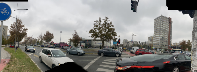
Error Location: Noticeable stitching artifact at the top edge, creating a black area where images failed to align.
- Reason: This issue likely arose in Step 1: Capture Overlapping Images. If the movement was inconsistent or too rapid, the overlapping regions between images could be misaligned, creating gaps or black spaces.
Error Location: Visible distortion of the building and the traffic light at the edges.
- Reason: This issue is related to Step 4: Estimate Initial Camera Parameters and Compute the Jacobian. Misalignment and improper initial camera parameter estimates can lead to perspective distortion, particularly on tall structures.
Error Location: Blending artifact along the ground, where the pavement and cars appear slightly misaligned.
- Reason: This likely occurred in Step 5: Apply Levenberg–Marquardt Optimization. Inaccurate Jacobian calculations or initial estimates can cause minor misalignments in overlapping areas, affecting horizontal objects like roads and pavements.
Image 2
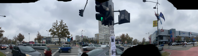
Error Location: Central pole appears misaligned and duplicated.
- Reason: This is due to errors in Step 3: Match Keypoints Across Images and Step 4: Estimate Initial Camera Parameters and Compute the Jacobian. The pole was likely matched incorrectly or duplicated due to false keypoints or poor initial alignment.
Error Location: Blurring and ghosting on the road and cars.
- Reason: This occurred during Step 2: Detect Features in Overlapping Regions and Step 6: Handle Outliers with Robust Cost Functions. Moving cars create challenges in detecting stable features, resulting in ghosting as the stitching algorithm struggles to handle moving objects.
Error Location: Sky shows artifacts where the edges do not align smoothly.
- Reason: Likely due to Step 7: Final Stitching. Issues in alignment and blending are particularly visible in areas without strong features, such as the sky, where there is insufficient detail for proper blending.
Image 3
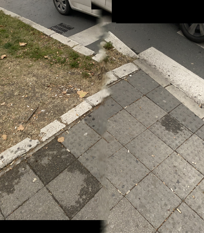
Error Location: Clear seam where the pavement is misaligned.
- Reason: This happened in Step 2: Detect Features in Overlapping Regions. The algorithm failed to detect enough distinctive features on the uniform pavement, resulting in alignment errors during stitching.
Error Location: Grass and sidewalk area have a visible discontinuity.
- Reason: This is likely an issue from Step 5: Apply Levenberg–Marquardt Optimization. Without accurate feature points and adjustments, flat, uniform areas can be challenging to align seamlessly.
Error Location: Duplicated and blurred area in the sidewalk section.
- Reason: This could be attributed to Step 3: Match Keypoints Across Images and Step 6: Handle Outliers with Robust Cost Functions. Outliers were not sufficiently filtered, causing mismatched keypoints that resulted in duplication.
Image 4
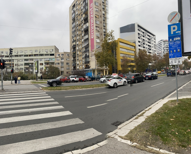
Error Location: Visible seam in the building structure, leading to distortion.
- Reason: This error occurred during Step 4: Estimate Initial Camera Parameters and Compute the Jacobian. Buildings with sharp, linear edges are susceptible to misalignment when initial parameters are inaccurate.
Error Location: Blurring of cars along the seam.
- Reason: Moving objects like cars pose issues in Step 6: Handle Outliers with Robust Cost Functions. The algorithm struggled to exclude outliers created by moving cars, causing ghosting.
Error Location: Misalignment on the crosswalk lines.
- Reason: This likely resulted from Step 5: Apply Levenberg–Marquardt Optimization. Accurate optimization and alignment are essential for horizontal elements like crosswalks, which were distorted due to insufficient parameter refinement.
Image 5
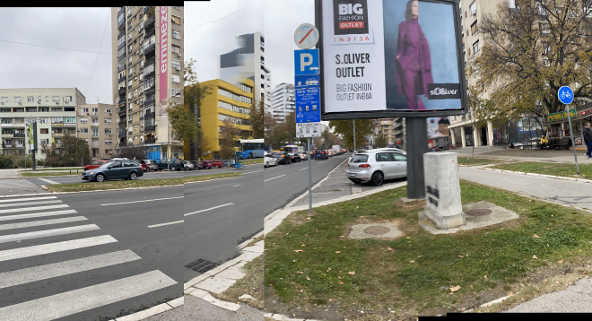
Error Location: Cars are visibly misaligned and duplicated.
- Reason: The errors here stem from Step 2: Detect Features in Overlapping Regions and Step 3: Match Keypoints Across Images. Moving cars lead to inconsistent keypoint matching, resulting in duplication.
Error Location: Distortion in the building with the pink banner.
- Reason: Likely due to Step 4: Estimate Initial Camera Parameters and Compute the Jacobian. Poor initial camera parameter estimation leads to distortion, especially in vertical structures.
Error Location: Blurred and inconsistent alignment along the sidewalk and curb.
- Reason: This problem occurred in Step 7: Final Stitching. The blending process failed to align these regions smoothly due to insufficient feature detection on uniform surfaces.
Step 1: Capture Overlapping Images#
Start by slowly moving the iPhone horizontally across the scene, allowing the camera to capture overlapping sections. This overlap provides reference points for stitching.
Errors and Fixes: If movement is too fast, motion blur can interfere with feature detection. Moving at a consistent, slow pace prevents this error.
Step 2: Detect Features in Overlapping Regions#
The iPhone uses algorithms like SIFT, SURF, or ORB to detect distinct features across the images. Examples include edges of buildings, streetlights, and other visually distinct objects. These keypoints act as anchors for aligning each image section.
Errors and Fixes: Homogeneous surfaces, such as a blank wall of the same color and without depth variation (2D), may lack sufficient features, leading to gaps in alignment. Using dense feature detection or switching to a different location can help mitigate this issue.
Step 3: Match Keypoints Across Images#
With features detected, the iPhone matches keypoints between overlapping images. For instance, the same streetlight edge is identified in two adjacent images, allowing them to align. The matching process relies on descriptors created by the feature detection algorithms.
Errors and Fixes: False matches can occur in repetitive patterns. RANSAC removes outliers by keeping only points that fit a transformation model.
Step 4: Estimate Initial Camera Parameters and Compute the Jacobian#
Using the iPhone’s accelerometer and gyroscope data, initial estimates for camera positions are set up. Bundle adjustment begins by calculating the Jacobian matrix, which approximates how each feature’s position changes based on slight variations in the camera position and orientation.
Errors and Fixes: Incorrect initial estimates lead to poor alignment. Calculating multiple initial estimates and choosing the best fit can improve accuracy.
Step 5: Apply Levenberg–Marquardt Optimization#
With the Jacobian computed, the iPhone uses the Levenberg–Marquardt algorithm to refine camera positions and keypoint locations iteratively. This minimizes misalignment by balancing between gradient descent and Gauss-Newton, adjusting parameters to reduce reprojection error.
Errors and Fixes: LM can converge to a local minimum, creating artifacts. Using good initial estimates and adjusting \(\lambda \) dynamically prevents early convergence on incorrect solutions.
Step 6: Handle Outliers with Robust Cost Functions#
The algorithm checks for outliers, such as moving objects (e.g., a passing car). By using robust cost functions, such as Huber or Tukey loss functions, the iPhone down-weights these points, ensuring they do not influence the alignment significantly. This improves the overall accuracy of the panoramic stitching.
Errors and Fixes: Outliers can skew results if not handled. Huber and Tukey loss functions help prevent outliers from heavily impacting the optimization.
Step 7: Final Stitching#
Once the camera parameters and keypoint locations are optimized, the iPhone combines the images into a single panoramic photo. The minimized reprojection error results in a seamless, aligned panorama with minimal visible seams or ghosting effects.
Errors and Fixes: Ghosting can occur if alignment is imperfect. Adjusting keypoint weights and smoothing transitions helps to reduce ghosting artifacts.
Theory#
Feature Detection Algorithms#
In panoramic photography, feature detection is crucial for identifying keypoints across multiple images. These keypoints serve as reference points for alignment and stitching. Commonly used algorithms are SIFT, SURF, and ORB, each providing unique benefits for detecting features invariant to scale, rotation, and translation. However, errors such as mismatches and insufficient features in homogeneous areas can occur, impacting alignment accuracy.
SIFT (Scale-Invariant Feature Transform)#
Scale-Space Creation: A Gaussian scale-space is created by progressively blurring the image at different scales.
Difference of Gaussians (DoG): DoG images are computed by subtracting adjacent scales, enhancing corners and edges.
Keypoint Detection: Local extrema in the DoG images are selected as keypoints, ensuring scale invariance.
Orientation Assignment: Keypoints are assigned dominant orientations based on local gradients, achieving rotation invariance.
Descriptor Generation: A 128-dimensional descriptor is generated by summarizing gradient information around each keypoint.
Errors and Fixes: In feature-poor regions, such as uniform textures or low-contrast areas, SIFT may struggle to identify distinctive keypoints, resulting in alignment issues. Using a robust detector like SIFT with dense sampling in such areas helps mitigate this problem.
SURF (Speeded-Up Robust Features)#
Integral Images and Scale-Space: SURF uses integral images to approximate Gaussian blurring, making it faster.
Hessian Matrix for Keypoint Detection: The determinant of the Hessian matrix identifies keypoints.
Orientation Assignment: Haar wavelet responses around each keypoint determine the dominant orientation.
Descriptor Generation: SURF creates a 64-dimensional descriptor based on Haar wavelet responses in a 4x4 grid around each keypoint.
Errors and Fixes: SURF can be affected by repetitive patterns, leading to false matches. RANSAC can be applied to filter out these mismatches.
ORB (Oriented FAST and Rotated BRIEF)#
FAST Keypoint Detection: ORB detects corners using the FAST algorithm, suitable for real-time applications.
Orientation Assignment: The intensity centroid method assigns orientation to each keypoint.
BRIEF Descriptor: A binary descriptor created by comparing pixel intensities around the keypoint, allowing for fast matching.
Errors and Fixes: ORB’s binary descriptors are susceptible to lighting changes, which can introduce mismatches. Adjusting image brightness or contrast can enhance ORB’s matching accuracy.
Bundle Adjustment and Optimization#
Bundle adjustment optimizes camera parameters and 3D keypoint locations to minimize reprojection error. This process is essential for accurate stitching in panoramas and 3D reconstructions. Errors due to linear Jacobian assumptions can arise if camera movement is non-linear, leading to stitching artifacts.
Jacobians in Panoramic Photography#
The Jacobian matrix represents the partial derivatives of projected 2D points with respect to camera and keypoint parameters. In panoramic photography, it calculates adjustments to align overlapping images. However, non-linear movements can make Jacobian approximations inaccurate, causing misalignment. Using adaptive optimization techniques helps correct these errors.
Optimization Techniques in Bundle Adjustment#
Levenberg–Marquardt (LM): Combines Gauss-Newton and gradient descent. It solves the system \((J^T J + \lambda I) \Delta = -J^T \epsilon \), where \(\lambda \) balances between the two methods. If the error decreases, \(\lambda \) is reduced; if it increases, \(\lambda \) is increased.
Gauss-Newton: An iterative approach using the first-order Hessian approximation, typically faster but less stable than LM in highly non-linear cases.
Conjugate Gradient (CG) Methods: Efficient for large, sparse problems without requiring explicit matrix inversion.
Sparse Bundle Adjustment (SBA): Optimized for sparse matrices, particularly useful for large datasets in bundle adjustment.
RANSAC (Random Sample Consensus)#
RANSAC is an iterative method used to estimate parameters of a model from a dataset that contains outliers. In feature matching, RANSAC helps identify and remove mismatched keypoints by fitting a transformation model and iteratively testing which matches conform to the model.
Steps of RANSAC:
Select a Random Subset: Choose a small subset of keypoints.
Estimate Model Parameters: Fit a transformation model (e.g., homography) to the subset.
Count Inliers: Test all points against the model, counting the points that fit within a threshold (inliers).
Repeat: Repeat for a set number of iterations or until the inlier count is satisfactory.
Choose Best Model: Use the model with the highest inlier count to retain only matches that are consistent with the transformation.
Huber and Tukey Loss Functions#
To handle outliers during optimization, robust cost functions like Huber and Tukey loss functions are applied. These functions down-weight outliers, reducing their impact on the final result.
Huber Loss Function: Transitions from quadratic to linear loss for large residuals, which helps prevent outliers from overly influencing the adjustment. Mathematically, it is defined as:
\[ \rho(x) = \begin{cases} x^2 & \text{for } |x| \leq \delta \ \delta (2|x| - \delta) & \text{for } |x| > \delta \end{cases} \]
where \( \delta \) is a threshold parameter.
Tukey Loss Function: Completely eliminates the influence of residuals beyond a certain threshold, which makes it very robust to strong outliers. Its formulation is:
\[ \rho(x) = \begin{cases} \delta^2 \left(1 - \left(1 - \frac{x^2}{\delta^2}\right)^3\right) & \text{for } |x| \leq \delta \ \delta^2 & \text{for } |x| > \delta \end{cases} \]